An intuitive understanding of variational autoencoders without any formula

Note from 2026. Diffusion models have largely eclipsed VAEs for photorealistic generation. The post is still worth reading if you want an intuitive grip on latent-variable models, the ELBO, and the reparameterization trick, all three show up everywhere downstream (diffusion, flow matching, modern variational inference, posterior sampling in RL, even parts of LLM alignment). VAEs are the cleanest small example of those ideas. Treat this as a gateway, not a state-of-the-art reference.

The short version. A plain autoencoder learns to compress and reconstruct, but its latent codes are not a distribution you can sample from, so it can’t generate new data. A variational autoencoder fixes that by forcing the latent code to come from a learned probability distribution \u2014 and the machinery that makes this work (ELBO, reparameterization, amortised inference) is the same machinery underneath diffusion, flow matching, and modern variational inference. This post is the intuition for all of it, in words and pictures.

I love the simplicity of autoencoders as a very intuitive unsupervised learning method. They are in the simplest case, a three layer neural network. In the first layer the data comes in, the second layer typically has smaller number of nodes than the input and the third layer is similar to the input layer. These layers are usually fully connected with each other. Such networks are called auto-encoders since they first “encode” the input to a hidden code and then “decode” it back from the hidden representation. They can be trained by simply measuring the reconstruction error and back-propagating it to the network’s parameters. If you add noise to the input before sending it through the network, they can learn better and in that case, they are called denoising autoencoders. They are useful because they help with understanding the data by trying to extract regularities in them and can compress them into a lower dimensional code.

alt text

A typical autoencoder can usually encode and decode data very well with low reconstruction error, but a random latent code seems to have little to do with the training data. In other words the latent code does not learn the probability distribution of the data and therefore, if we are interested in generating more data like our dataset a typical autoencoder doesn’t seem to work as well. There is however another version of autoencoders, called “variational autoencoder - VAE” that are able to solve this problem since they explicitly define a probability distribution on the latent code. The neural network architecture is very similar to a regular autoencoder but the difference is that the hidden code comes from a probability distribution that is learned during the training. Since it is not very easy to navigate through the math and equations of VAEs, I want to dedicate this post to explaining the intuition behind them. With the intuition in hand, you can understand the math and code if you want to.

I start with a short history. Over the past two decades, researchers have been trying to develop a framework for probabilistic modeling that explicitly conveys the assumption being made about the data. The result of this effort has been probabilistic graphical models that combine ideas from graph theory and probability theory. Graphical models use a graph representation to encode a probability distribution over a set of random variables. The graph is a very flexible language that admits composability for building arbitrarily complex models and provides a set of tools for reasoning (inference) about different nodes. (There is a companion post on graphical models if you want the broader framing; this one zooms in on one particular graphical model that turns out to be unusually useful.)

Using graphical models language we can explicitly articulate the hidden structure that we believe is generating the data. For example, if we believe that there is a hidden variable $z_{i}$ for each observable data point $x_{i}$ that is causing the data, we can make a model like this:

Since data points, $X$ , are observed while the $Z$ nodes are unknown, we want to “infer” the hidden variables $z_{i}$ from known data points. The solid line shows the data generation path and the dashed line shows the inference path.

Reasoning (inference) about hidden variables in probabilistic graphical models has traditionally been very hard and only limited to very restricted graph structures. This issue had significantly limited our ability to build interesting models and perform reasoning on them in the past. However, in the past few years there have been some very exciting developments that have enabled us to perform approximate reasoning with scalable algorithms like stochastic gradient descent. This has triggered another wave of interest in graphical models.

Recent developments come from the idea that directed graphical models can represent complex distributions over data while deep neural nets can represent arbitrarily complex functions. We use deep neural networks to parameterize and represent conditional distributions. Variational autoencoders are the result of the marriage of these two set of models combined with stochastic variational and amortized inference.

A variational autoencoder is essentially a graphical model similar to the figure above in the simplest case. We assume a local latent variable, $z_{i}$ for each data point $x_{i}$ . The inference and data generation in a VAE benefit from the power of deep neural networks and scalable optimization algorithms like SGD.

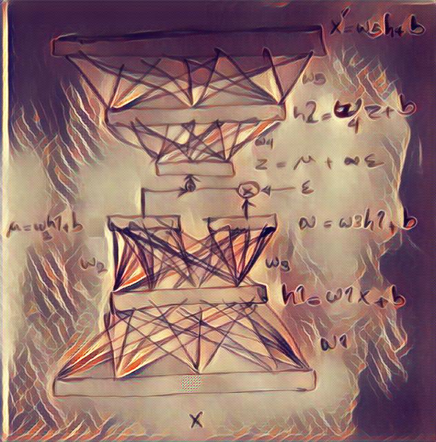
As can be seen from the picture above, in a VAE, the encoder becomes a variational inference network that maps the data to the a distribution for the hidden variables, and the decoder becomes a generative network that maps the latent variables back to the data. Since the latent variable is actually a probability distribution, we need to sample the hidden code from its distribution to be able to generate data.

alt text

In order to be able to use stochastic gradient descent with this autoencoder network, we need to be able to calculate gradients w.r.t. all the nodes in the network. However, latent variables, $z$ , in a graphical model are random variables (distributions) which are not differentiable. Therefore, to make it differentiable, we treat the mean and variance of the distribution as simple deterministic parameters and form the sample as $z = μ + σ ⊙ ϵ$ where $ϵ$ is drawn from a standard normal (i.e. we multiply the standard deviation by a noise sample and add the mean). By parameterizing the hidden distribution this way, we can back-propagate the gradient to the parameters of the encoder and train the whole network with stochastic gradient descent. This procedure will allow us to learn mean and variance values for the hidden code and it’s called the “re-parameterization trick”. It is important to appreciate the importance of the fact that the whole network is now differentiable. This means that optimization techniques can now be used to solve the inference problem efficiently.

In classic neural networks we train by minimising a pixel-wise error like mean squared error. That is fine for a VAE too, MSE is the log-likelihood under a Gaussian output, and cross-entropy is the log-likelihood under a Bernoulli output. What changes in a VAE is that the reconstruction loss is only half of the objective. The other half is a KL divergence that measures how far the approximate posterior $q (z ∣ x)$ strays from the prior $p (z)$ , and that acts as a regulariser on the latent space. The true quantity we would like to minimise, $K L [q (z ∣ x) ∥ p (z ∣ x)]$ , is intractable because $p (z ∣ x)$ is unknown; some simple algebra rewrites it as $lo g p (x)$ minus a tractable quantity called the ELBO (evidence lower bound). Because $lo g p (x)$ does not depend on the parameters of $q$ , minimising the intractable KL is equivalent to maximising the ELBO, and the ELBO decomposes exactly into reconstruction log-likelihood plus the KL regulariser above. That is the whole objective.

Here is a high level pseudo-code for the architecture of a VAE to put things into perspective:


network= {

  # encoder
  encoder_x = Input_layer(size=input_size, input=data)
  encoder_h = Dense_layer(size=hidden_size, input= encoder_x)

  # the re-parameterized distributions that are inferred from data 
  z_mean = Dense(size=number_of_distributions, input=encoder_h)
  z_variance = Dense(size=number_of_distributions, input=encoder_h)
  epsilon= random(size=number_of_distributions)

  # decoder network needs a sample from the code distribution
  z_sample= z_mean + exp(z_variance / 2) * epsilon

  #decoder
  decoder_h = Dense_layer(size=hidden_size, input=z_sample)
  decoder_output = Dense_layer(size=input_size, input=decoder_h)
}

cost={
  reconstruction_loss = input_size * crossentropy(data, decoder_output)
  kl_loss = - 0.5 * sum(1 + z_variance - square(z_mean) - exp(z_variance))
  cost_total= reconstruction_loss + kl_loss
}

stochastic_gradient_descent(data, network, cost_total)

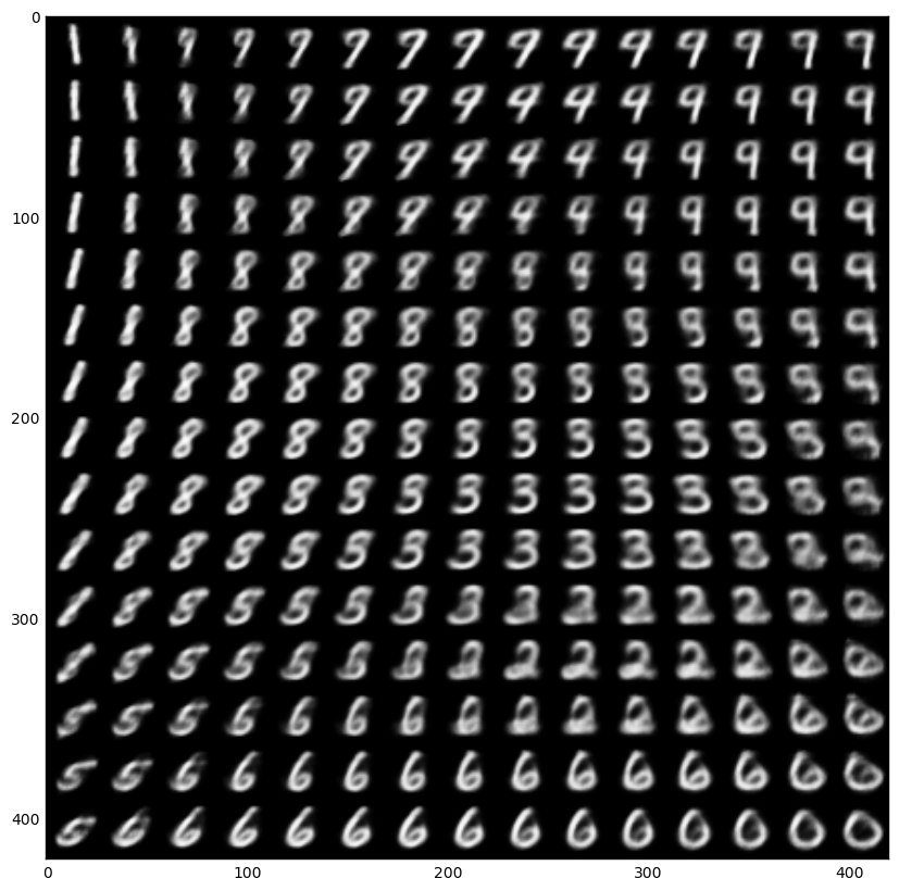
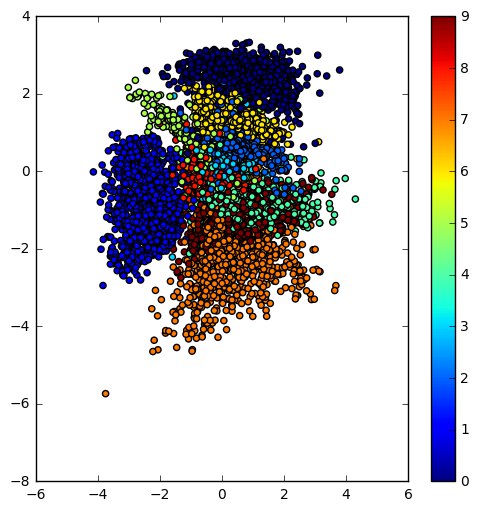
Now that the intuition is clear, here is a Jupyter notebook for playing with VAEs, if you like to learn more. The notebook is based on this Keras example. The resulting learned latent space of the encoder and the manifold of a simple VAE trained on the MNIST dataset are below.

VAE Latent space | VAE generated samples

Side note 1:

The ELBO is determined from introducing a variational distribution q, on lower bound on the marginal log likelihood, i.e. $lo g p (x) = lo g \int_{z} p (x, z) * \frac{q ( z ∣ x )}{q ( z ∣ x )}$ . We use the log likelihood to be able to use the concavity of the $lo g$ function and employ Jensen’s inequality to move the $lo g$ inside the integral i.e. $lo g p (x) > \int_{z} lo g (p (x, z) * \frac{q ( z ∣ x )}{q ( z ∣ x )})$ and then use the definition of expectation on $q$ (the nominator $q$ goes into the definition of the expectation on $q$ to write that as the ELBO) $lo g p (x) > E L B O (z) = E_{q} [- lo g q (z ∣ x) + lo g p (x, z)]$ . The difference between the ELBO and the marginal $p (x)$ which converts the inequality to an equality is the distance between the real posterior and the approximate posterior i.e. $K L [q (z ∣ x) ∣ p (z ∣ x)]$ . Alternatively, the distance between the ELBO and the KL term is the log-normalizer $p (x)$ . Replace the $p (z ∣ x)$ with Bayesian formula to see how.

Now that we have a defined a loss function, we need the gradient of the loss function, $\nabla E_{q} [- lo g q (z ∣ x) + lo g p (x, z)]$ to be able to use it for optimization with SGD. The gradient isn’t easy to derive analytically but we can estimate it with the score-function (REINFORCE / log-derivative) estimator, which samples $z \sim q (z ∣ x)$ and weights the integrand by $\nabla lo g q (z ∣ x)$ . This estimator is unbiased but generally exhibits large variance, because the $\nabla lo g q$ factor can be very large at rare samples.

This is where the re-parameterization trick we discussed above comes in. We assume that the random variable $z$ is a deterministic function of $x$ and a known $ϵ$ ( $ϵ$ are iid samples) that injects randomness $z = g (x, ϵ)$ . This re-parameterization converts the undifferentiable random variable $z$ , to a differentiable function of $x$ and a decoupled source of randomness. Therefore, using this re-parameterization, we can estimate the gradient of the ELBO as $\nabla E_{ϵ} [- lo g q (g (x, ϵ) ∣ x) + lo g p (x, g (x, ϵ))]$ . This estimate to the gradient has empirically shown to have much less variance and is called “Stochastic Gradient Variational Bayes (SGVB)”. SGVB is sometimes called a black-box inference method (like the score-function estimator) because it doesn’t care what functions we use in the generative and inference network. It only needs to be able the calculate the gradient at samples of $ϵ$ . We can use SGVB with a separate set of parameters for each observation however that’s costly and inefficient. We usually choose to “amortize” the cost of inference with deep networks (to learn a single complex function for all observations instead). All the terms of the ELBO are differentiable now if we choose deep networks as our likelihood and approximate posterior functions. Therefore, we have an end-to-end differentiable model. Following depiction shows amortized SGVB re-parameterization in a VAE.

Simple VAE structure with reparameterization

side note 2:

Note that in the above derivation of the ELBO, the first term is the entropy of the variational posterior and second term is log of joint distribution. However we usually write joint distribution as $p (x, z) = p (x ∣ z) p (z)$ to rewrite the ELBO as $E_{q} [lo g p (x ∣ z) + K L (q (z ∣ x) ∣ p (z))]$ . This derivation is much closer to the typical machine learning literature in deep networks. The first term is log likelihood (i.e. reconstruction cost) while the second term is KL divergence between the prior and the posterior (i.e a regularization term that won’t allow posterior to deviate much from the prior). Also note that if we only use the first term as our cost function, the learning with correspond to maximum likelihood learning that does not include regularization and might overfit.

Side note 3: KL direction, posterior collapse, and mode coverage

KL divergence is not symmetric: $K L (P ∥ Q) = E_{P} [lo g P (x) - lo g Q (x)]$ , and the direction you choose has real consequences. In minimising $K L (p ∥ q)$ (the mode-covering direction), $q$ is penalised wherever $p$ has mass but $q$ does not, so $q$ smears across every mode of $p$ ; this is the direction supervised maximum likelihood uses. In minimising $K L (q ∥ p)$ (the mode-seeking direction), $q$ is penalised wherever $q$ has mass but $p$ does not, so $q$ prefers to sit on a single mode of $p$ and leave the others alone.

A VAE actually minimises $K L [q (z ∣ x) ∥ p (z ∣ x)]$ , the mode-seeking direction, over latent posteriors, not over data. This is what motivates the common VAE failure mode of posterior collapse: the approximate posterior $q (z ∣ x)$ drifts to match the prior $p (z)$ exactly, the KL term in the ELBO goes to zero, and the latent becomes uninformative about $x$ . This is a different phenomenon from GAN-style mode collapse (where the generator covers only a few modes of the data distribution); the two are often conflated because both are sometimes called “mode collapse” in casual discussion. VAE outputs do also tend to be blurry, but that is a separate consequence of maximum-likelihood training with a Gaussian/Bernoulli decoder, not of the KL direction.

alt text

references:

[1] Kingma, Diederik P., and Max Welling. “Auto-encoding variational Bayes.” arXiv preprint arXiv:1312.6114 (2013).

[2] Rezende, Danilo Jimenez, Shakir Mohamed, and Daan Wierstra. “Stochastic backpropagation and approximate inference in deep generative models.” arXiv preprint arXiv:1401.4082 (2014).

[3] https://www.cs.princeton.edu/courses/archive/fall11/cos597C/lectures/variational-inference-i.pdf